Often in science we want to be able to quantify the effect of an action on some outcome. For example, perhaps we are interested in estimating the effect of a drug on blood pressure. While it is easy to show whether or not taking the drug is associated with an increase in blood pressure, it is surprisingly difficult to show that taking the drug actually caused an increase (or decrease) in blood pressure.

Causal inference is the field of statistics (or economics, depending on who you ask) that is concerned with estimating the causal effect of a treatment.[^check]

The fundamental problem of causal inference

Why is estimating a causal effect difficult? To put it simply, the fundamental problem is that we can never actually observe a causal effect. The causal effect is defined to be the difference between the outcome when the treatment was applied and the outcome when it was not. This difference is a fundamentally unobservable quantity. For any individual, we can only ever observe their blood pressure either in the situation (1) when they take the drug or (2) when they don’t. We can never observe both since an individual cannot simultaneously both take the drug and not take the drug.

Introducing some notation, the outcome we would observe for an individual had they received the treatment (in which case we set the treatment indicator, \(T = 1\)) is denoted \(Y(1)\) and the outcome for an individual had they not received treatment (treatment indicator, \(T = 0\)) is denoted \(Y(0)\).

The outcome that we actually observe (\(Y\)) can be written as a linear combination of these quantities:

\[Y = T \times Y(1) + (1 - T) \times Y(0).\]

Since we can only ever observe one of the two potential outcomes, \(Y(1)\) or \(Y(0)\), how can we estimate the causal effect (i.e. the expected difference between the two potential outcomes)?

\[\tau = E[Y(1) - Y(0)]\]

This is a very unique type of missing data problem, and the key to estimating casual effects lies in understanding the principles of randomized experiments.

Confounders are the worst!

Suppose that we have conducted a randomized experiment in which we measure some outcome (say mortality) within two groups, treated and untreated, into which individuals were randomly assigned. In this case, the random assignment of treatment means that there should, on average, be no significant differences between the treated and untreated groups. Thus, any difference in mortality that we observe between the treated group and the untreated group must be due to the treatment itself (as this is the only thing that differs between the treated and untreated groups).

One of the primary problems that arise when attempting to estimate average causal effects in an observational study (i.e. a study in which the individuals assign themselves into a treatment group, e.g. because they themselves choose to smoke or not, rather than a scientist choosing for them) is that there may exist differences between the treated group and the untreated group, other than the treatment itself, such as gender (males are more likely to smoke).

Why is this a problem? Basically, if there is something other than the treatment that differs between the treated and untreated groups, then we cannot conclusively say that any difference observed in mortality (or any other outcome of interest) between the two groups is due solely to the treatment. Such a difference could also plausibly be due to these other variables that differ between these groups. These variables that differ between the treatment and control groups are called confounders if they also influence the outcome.

For a simplified example, it is known that males are more likely to smoke than females, but males are also more likely to die young as a result of other general risk-raking behavior. In this case, if we notice a difference in mortality between smokers and non-smokers, we cannot be sure that this difference is due to the smoking rather than the fact that the group of smokers consists more of males than the control group and subsequently (as a result of the risk-taking behavior, rather than just the smoking) the treatment group has a higher mortality rate than the untreated group. In this case, the higher mortality rate among smokers has nothing to do with (or at least is not entirely due to) the smoking itself, but rather is to do gender discrepancies and the differences in risk-taking behaviors afforded by such a discrepancy.

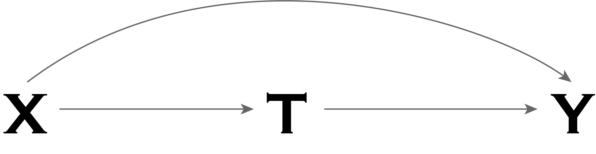
In the graph below, our example corresponds to the outcome, \(Y\), mortality; the treatment, \(T\), smoking, and the confounder, \(X\), gender.

Note that if gender differed between the treatment and untreated group (e.g. smokers vs non-smokers), but had no association with the outcome (e.g. mortality), then gender would not be considered a confounder (as it would not be a common cause of treatment the and outcome).

Clearly estimating causal effects in the presence of confounders is going to be a problem!

So when is our estimator “identifiable”?

The goal is to estimate the expected potential outcomes in (1) the situation that all individuals in the entire population (of which our study is a small subset) were assigned the treatment, and (2) the situation that none of the individuals in the population were assigned the treatment, and take the difference between these two quantities:

\[\tau = E[Y(1)] - E[Y(0)]\]

This quantity is referred to as the population average causal effect.

Typically, the way we would want to estimate this quantity is using the conditional sample averages:

\[\widehat{\tau} = \widehat{E}[Y | T = 1] - \widehat{E}[Y | T = 0].\]

Note that while \(E[Y(1)]\) referred to the expected outcome in the hypothetical situation that everyone in the population was assigned to treatment, \(E[Y | T = 1]\) refers to the expected outcome for all individuals in the population who are actually assigned to treatment.

where we take the observed average outcome of all treated individuals in our study subset and subtract the observed average outcome of all untreated individuals in our study subset.

However, this quantity is only an unbiased estimator of the true average causal effect, \(\tau\), when the following identifiability conditions hold:

The treated and untreated individuals are exchangeable wherein the assignment of treatment does not depend on the potential outcomes (i.e. that there are no unmeasured confounders that are a common cause of both treatment and the outcome):¹ \[Y(1), Y(0) \perp T\]
The probability of receiving every level of treatment is positive for every individual, known as positivity. This means that there is no individual for whom receiving the treatment is impossible (and vice versa for the control).
The treatment is defined unambiguously, i.e. that the potential outcome that corresponds to the treatment that the individual actually received is “factual”. This is called consistency. In particular, this is often taken to mean that there are not multiple versions of treatment, i.e. that if an individual, \(j\), received treatment \(t\) by means (route, condition, etc) \(k\), then consistency means that \[Y_j = Y_j(t, k)~~ \textrm{ if }~~ t = T_j ~\textrm{ no matter the value of } k\] Cole and Frangakis from UNC provide a nice discussion on consistency if you’re interested in understanding this condition more deeply.

The key is that the value of \(E[Y | T = 1] - E[Y | T = 0]\) is only equal to the causal effect, \(E[Y(1) - Y(0)]\) if there are no confounders present, measured or unmeasured (and the other identifiability assumptions of positivity and consistency hold). Recall that a confounder can be thought of a variable, \(X\) that differs between the treatment (\(T = 1\)) and control (\(T = 0\)) groups and also influences the outcome, \(Y\). That is, a confounder is a common cause of both the treatment and the outcome.

Basically, if there are confounders present, then the treatment and control groups are no longer exchangeable. In particular, the expected outcome for the individuals that were actually treated, \(E[Y | T = 1]\), may not be equal to the potential outcome under treatment for the entire population (regardless of actual treatment assignment), \(E[Y(1)]\).

Dealing with measured confounding

If there are confounders present, then the quantity, \(E[Y | T = 1] - E[Y | T = 0]\), provides a measure of association (rather than causation). Fortunately, in the situation where all confounders are measured, there do exist methods for adjusting the estimate so that we can actually estimate a causal effect.

If all confounders are measured, and we can assume that exchangeability holds within the strata dictated by the confounders (this is called conditional exchangeabiliity) then we can still estimate the causal effect using methods that eliminate the confounding. Conditional exchangeability essentially means that, even if there are confounding variables that differ between the treatment and control groups that affect the outcome, if we only look at individuals who take a single value for that confounding variable, then the treatment assignment within each strata is “as if” random. We can then replace the first ignorability condition with the following:

The treated and untreated individuals are exchangeable wherein the assignment of treatment depends only on the measured covariates, \(X\) (i.e. that there are no unmeasured confounders and no informative censoring). This is commonly known as ignorability, and is typically presented as \[Y(1), Y(0) \perp T | X\] (this is technically strong ignorability; ignorability actually refers to the weaker restriction where treatment assignment mechanism can be written in terms of \(X\), \(T\) and the observed \(Y\) without dependence on the missing outcomes).

Under this condition (as well as positivity and consistency), there are alternative versions of the estimator, \(\hat{E}[Y|T = 1] - \hat{E}[Y|T = 0]\) that we can use to obtain an unbiased estimate of the causal effect.

The most common methods for adjusting the estimator to eliminate the confounding are:

Matching, restriction, and stratification (note that an example of stratification is adjustment via regression): methods that exploit conditional exchangeability in subsets defined by some confounder to estimate the association between treatment and outcome in those subsets only.
Standardization, inverse-probability (or inverse-propensity) weighting, and G-estimation: methods that exploit conditional exchangeability in subsets defined by some confounder to estimate the causal effect in the entire population or in any subset of the population.

However, note that we must be careful when selecting/identifying confounders on which to adjust, since in certain circumstances, conditioning on non-confounders can actually introduce confounding into the problem! As such, subject-matter knowledge becomes necessary to identify possible confounders. In observational studies, causal inference relies on the uncheckable assumption of no unmeasured confounding or of conditional exchangeability.

What about unmeasured confounders?

If there exist unmeasured confounders that may be a common cause of both the outcome and the treatment, then it is impossible to accurately estimate the causal effect. Period. Moreover, it is impossible to actually check whether there exists unobserved confounding. Everything relies on the validity of your assumptions. Sorry about that.

Footnotes

I know the \(\perp\) symbol means perpendicular not independent, but I couldn’t be bothered figuring out how to add LaTeX preamble to markdown to define the double vertical line independent symbol. Don’t judge me!↩︎