In my previous post, I introduced causal inference as a field interested in estimating the unobservable causal effects of a treatment: i.e. the difference between some measured outcome when the individual is assigned a treatment and the same outcome when the individual is not assigned the treatment.
If you’d like to quickly brush up on your causal inference, the fundamental issue associated with making causal inferences, and in particular, the troubles that arise in the presence of confounding, I suggest you read my previous post on this topic.
Confounding and idenitifiability
Recall that the causal estimand is identifiable when (1) exchangeability/ignorability, (2) consistency and (3) positivity all hold. This means that the causal effect can be unbiasedly estimated using the estimand, \[\hat{\tau} = \frac{1}{n_T}\sum_{i : T_i = 1} y_i - \frac{1}{n_C}\sum_{i:T_i = 0}y_i.\] where \(n_T\) and \(n_C\) are the number of individuals in the treated and control groups, respectively. This is the difference between the average treated and control outcomes.
In the presence of confounding, the exchangeability assumption is false, implying that the estimand above is not unbiased for the true population average causal effect.
Under the stronger condition of conditional exchangeability, wherein exchangeability holds within each strata of the confounding variables (i.e. \(Y(1), Y(0) \perp T | X\)), then there are methods that can be used to eliminate confounding and estimate the causal effect.
In this post, I will discuss one such method, the inverse-probability method, for removing (or adjusting for) confounding.
The issue is that we can never truly know whether or not we have actually removed all confounding… but we will ignore this for now, and assume that we know each of the confounders in our data and that there are no unmeasured confounders.
Inverse probability weighting
Inverse-probability weighting removes confounding by creating a “pseudo-population” in which the treatment is independent of the measured confounders.
Weighting procedures are not new, and have a long history being used in survey sampling. The idea of weighting observations in a survey sample is based on the idea that the sample surveyed is not quite representative of the broader population. The goal is to make the sample look more like the population. To do so, you can add a larger weight to the individuals who are underrepresented in the sample and a lower weight to those who are over-represented (e.g. if the population is 50% female, but your sample is only 35% female, you would add a larger weight to the female respondents). By the way to “assign a weight”, “re-weight”, or “add a weight” to an individual simply means to multiply their outcome by the weight in question.
This idea of re-weighting our sample in the context of estimating causal effects has a similar flavour, but it may take a bit of brain twisting to understand why, but let me phrase it as simply as I can in my current sleep deprived state:
Suppose that there are measurable differences between the control and treated groups. For example, perhaps younger males are much more likely to be in the treatment group than older males. Just because younger males are more likely to be in the treatment group, that doesn’t mean that all younger males will be in the treatment group. Some of these younger males, even though they were very similar to their peers in every measurable way, ended up in the control group. In this case, it would make sense that comparing the outcome of these few young males in the control group with the outcome of the many young males in the treatment group serves as a fairly good estimate of the causal effect for the subgroup of young males. So we could up-weight the young males who were placed in the control group and down-weight the young males who, as expected, were placed in the treatment group.
This is the basic idea behind inverse probability weighting. Individuals who were assigned to the treatment group even though they were much more likely to be assigned to the control group are a rare, and valuable breed. We want to give their outcomes as much weight as possible, whereas the much larger group of individuals who were placed in the expected treatment group need less weight, simply because we have much more information on individuals like this.
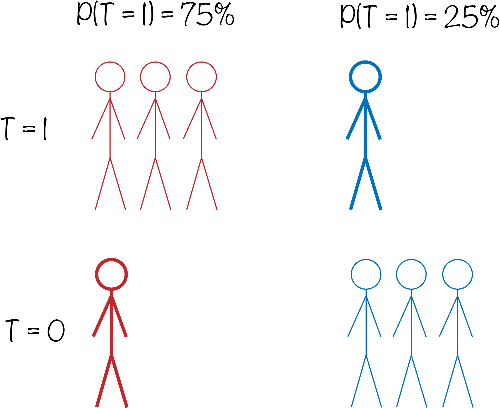
Suppose that there are two types of people. The first type has a 75% chance of receiving treatment, while the second type has only a 25% chance. If there are 4 people in each group, then we would expect that three of the people in the first group received treatment, while only one person from the second group would. If we wanted to estimate the causal effect (i.e. the difference in the average outcome between the first and second row), then it would be better if we could improve the treatment-control balance within each of the two treatment allocation groups. Thus, perhaps we could assign a weight of three to each of the single individuals in each group who were assigned to the less likely treatment class, (or alternatively a weight of 1/3 to each of the three individuals in each group who were assigned to the expected class).
This idea is demonstrated in the image below.
As implied by its name, inverse probability weighting literally refers to weighting the outcome measures by the inverse of the probability of the individual with a given set of covariates being assigned to their treatment (note that this doesn’t depend on whether or not the individual was in fact assigned to treatment).This quantity is known as the propensity score and is denoted
\[p(x) = P(T = 1 | X = x)\]
For treated individuals, we weight their outcome by \[w(x) = \frac{1}{p(x)},\]
whereas for control individuals, the weight is:
\[w(x) = \frac{1}{1 - p(x)}\]
Obviously unless we randomly assigned treatment with a set probability (as in the example above), we do not actually know the propensity score of each individual. What we do observe however, is which individuals were actually assigned to treatment, along with a number of measured covariates for each individual. The idea is that we can use these covariates as well as our observation of who received treatment to develop a logistic regression model that predicts the probability of treatment (propensity score).
Thus, in the presence of measured confounders, we can estimate the causal effect by IP-weighting the original estimator:
\[\begin{align*} \hat{\tau}^{\textrm{IP}} &= \frac{1}{n_T}\sum_{i : T_i = 1} \frac{Y_i}{\hat{p}(X_i)} - \frac{1}{n_C}\sum_{i:T_i = 0}\frac{Y_i}{1 - \hat{p}(X_i)} \\ & = \frac{1}{n}\sum_i^n \frac{T_iY_i}{\hat{p}(X_i)} - \frac{1}{n}\sum_i^n \frac{(1 - T_i)Y_i}{1 - \hat{p}(X_i)}. \end{align*}\]
where \(\hat{p}(x)\) is a logistic-regression based estimator of the propensity score.
To show that this quantity is unbiased for the original quantity we want to estimate, \(\tau = E[Y(1)] - E[Y(0)]\), it is sufficient to show that
\[E \left[ \frac{Y T}{p(X)}\right] = E[Y(1)], ~~~~~ \textrm{and} ~~~~~ E \left[ \frac{Y (1 - T)}{1 - p(X)}\right] = E[Y(0)]\] which is easy to see as follows:
\[\begin{align*} E \left[ \frac{Y ~T}{p(X)}\right] &= E \left[ E \left[ \frac{Y T}{p(X) }\Bigg| X\right] \right]\\ & = E \left[ E \left[ \frac{Y(1) ~T}{p(X)} \Bigg|X\right] \right]\\ & = E \left[ \frac{E [ Y(1) |X]~ E[T | X]}{p(X)} \right]\\ & = E \left[E [ Y(1) |X] \right]\\ & = E \left[ Y(1) \right]\\ \end{align*}\]
and similarly for the second equality.
Standardized IP-weighting
One common issue with IP-weighting is that individuals with a propensity score very close to 0 (i.e. those extremely unlikely to be treated) will end up with a horrifyingly large weight, potentially making the weighted estimator highly unstable.
A common alternative to the conventional weights that at least “kind of” addresses this problem are the stabilized weights, which use the marginal probability of treatment instead of \(1\) in the weight numerator.
For treated individuals, the stabilized weight is given by
\[w(x) = \frac{P(T = 1)}{p(x)} = \frac{P(T = 1)}{P(T = 1 | X = x)}\]
and for control individuals, the stabilized weight is \[w(x) = \frac{1 - P(T = 1)}{1 - p(x)} = \frac{1 - P(T = 1)}{1 - P(T = 1 | X = x)}\]
Note that whereas the original weights essentially doubles the sample size, these stabilized weights preserve the sample size.
Resources
Much of the information provided in this post can be found in the Causal Inference book by Miguel A. Hernan and James M. Robins.
Additional resources are the books Causal Inference for Statistics, Social, and Biomedical Sciences by Guido W. Imbens and Donald B. Rubin, and Mostly Harmless Econometrics by Joshua D. Angrist and Jörn-Steffen Pischke.